Basic Info

• link to paper.
• Yi, Xinyang, et al. “Sampling-bias-corrected neural modeling for large corpus item recommendations.” Proceedings of the 13th ACM Conference on Recommender Systems. 2019.

Summary

This paper proposed a framework to correct sampling-bias of in-bacth training loss of two-tower models. The paper present a simple algorithm to estimate the frequency of streaming data and through theoretical analysis and simulation, they show that this algorithm can work without requiring fixed item vocabulary, and is capable of producing unbiased estimation and being adaptive to item distribution change. And they apply the sampling-bias corrected modeling approach to build a large scale neural retrieval system for YouTube recommendations. And they claim that this system leads to improved recommendation quality for YouTube show by live A/B testings.

Sampled Softmax

Softmax is one of the most commonly used functions in designing models of a large output space. In order to speed up training, one technique that widely used is to sample a subset of classes. Bengio et al. [1] shows a good sampling distribution should be adaptive to model’s output distribution. Recently, Blance et al. [2] designs an efficient and adaptive kernel based sampling method. As paper point out, sampled softmax is not applicable to the case where label has content features, in this case, adaptive sampling still remains an open problem. Note that we can also use hierarchical softmax to speed up train and inference time, but it typically require a predefined tree structure based on certain categorical attributes.

Sampling-Bias

Suppose we have queries and items represented by feature vectors \(\{x_i\}^{N}_{i=1}\) and \(\{y_i\}^{N}_{i=1}\) respectively. Here \(x \in \mathcal{X}\) and \(y \in \mathcal{Y}\) are both mixtures of a wide variety of features. And we want to build two paramaterized functions: \(u: \mathcal{X} \times \mathbb{R}^{d} \mapsto \mathbb{R}^{k}\), \(v: \mathcal{Y} \times \mathbb{R}^{d} \mapsto \mathbb{R}^{k}\). These functions map model paramater \(\theta \in \mathbb{R}^{d}\) and features of query and candicates to a k-dimenisional embedding space. And we focus on a two-tower neural net architecture here illustrated by the figure below. The output of the model is a score (logit) which is just the inner product of two embeddings, namely,

\[s(x, y) = \langle u \left(x, \theta \right), v \left(y, \theta \right) \rangle\]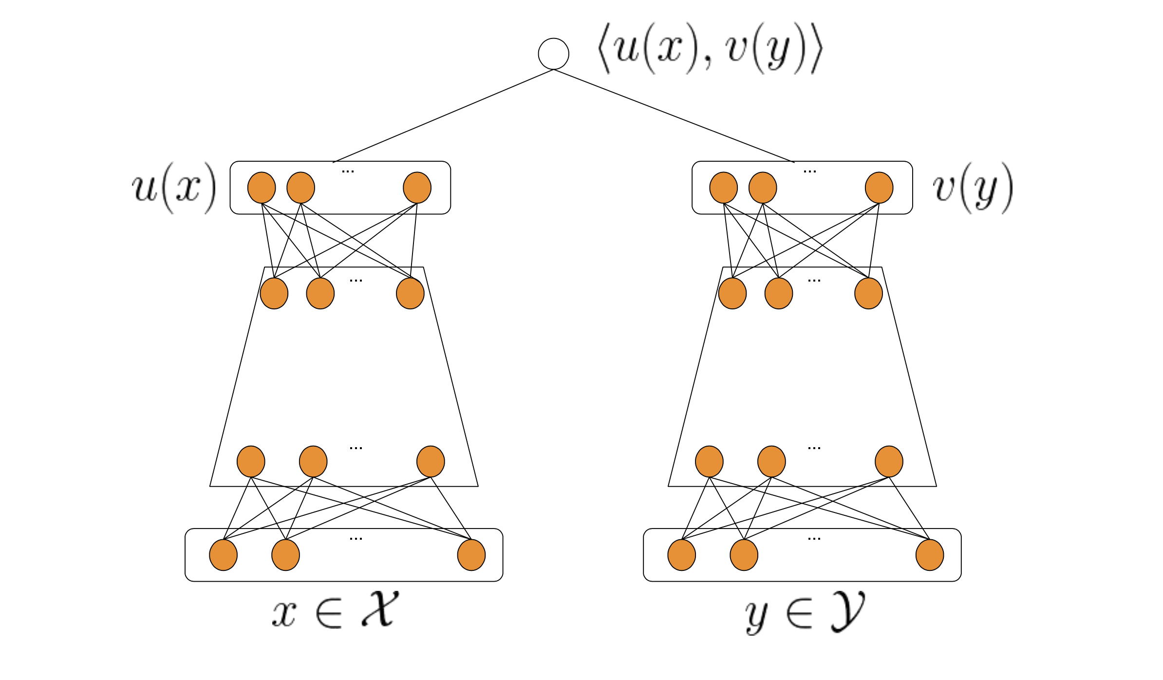

We want to learn the model parameter \(\theta\) from a training dataset of \(T\) examples, denoted by:

\[\mathcal{T} := \{ \left(x_i, y_i, r_i \right) \} ^{T}_{i=1}\]

Where \((x_i, y_i)\) denote the pair of query \(x_i\) and item \(y_i\), and \(r_i\) is the associated reward for each pair. Given a query \(x\), the probability distribution of picking the item \(y\) from \(M\) items \(\{ y_j \}^{M}_{j=1}\) is calculated by softmax function, i.e.,

\[\mathcal{P} \left( y \mid x; \theta \right) = \frac{e^{s \left( x, y \right)}}{\sum_{j \in [M]} e^{s \left(x, y_j \right)}}\]

We consider the following weighted log-likelihood as loos function by incorporating reward \(r_i\):

\[L_{T} \left( \theta \right) := -\frac{1}{T} \sum_{i \in [T]} {r_i \cdot \mathcal{P} \log \left( \left( y_i \mid x_i; \theta \right) \right)}\]

If the \(M\) is very large, one way to construct the partition function is to use a subset of items. And when dealing with streming data, we consider only use in-batch items [3] as negatives for all queries from the same batch. Precisely, given a mini-batch of \(B\) pairs \(\{ \left( x_i, y_i, r_i \right) \}^{B}_{i=1}\), for each \(i \in [B]\), the batch softmax is

\[\mathcal{P}_{B} \left( y_i \mid x_i; \theta \right) = \frac{ e^{s \left( x_i, y_i \right)} } { \sum_{j \in [B]} {e^{s \left( x_i, y_j \right)}} }\]

In-batch items are normally sampled from power-law distribution in target applications. As a result, popular items are overly penalized as negatives due to high probability of occurrence.

Correction

Inspired by the \(\log Q\) correction used in sampled softmax model [1], we correct each score \(s(x_i, y_j)\) by the following equation

\[s^{c} \left( x_i, y_j \right) = s \left( x_i, y_j \right) - \log p_j\]

Here \(p_j\) of denotes the sampling probability of item j in a random batch. With the correction, we have

\[\mathcal{P}^{c}_{B} \left( y_i \mid x_i; \theta \right) = \frac{ e^{s^{c} \left( x_i, y_i \right)} } { e^{s^{c} \left( x_i, y_i \right)} + \sum_{j \in [B], j \neq i}{e^{s^{c} \left( x_i, y_j \right)}} }\]

Then the final batch loss can be write as

\[L_{B} \left( \theta \right) := - \frac{1}{B} \sum_{i \in [B]} {r_i \cdot \log \left( \mathcal{P}^{c}_{B} \left( y_i \mid x_i; \theta \right) \right)}\]

Estimation Algorithm

We can convert the estimation of frequency \(p\) of an item to the estimation of \(\delta\), which denotes average number of steps between two consecutive hits of the item. We will use two array \(A, B\) with size \(H\) and a hash function \(h\) to design a novel algorithm to do the stream frequency estimation.

\[\begin{align*} B[h \left( y \right)] & \leftarrow (1 - \alpha) \cdot B[h \left( y \right)] + \alpha \cdot \left( t - A[h \left( y \right)] \right) \\ A[h \left( y \right)] & \leftarrow t \\ \end{align*}\]

Here \(t\) means at step \(t\). \(B\) contains the estimation of \(\delta\) of \(y\). Suppose the number of steps of two consecutive hits folllow a distribution represented of a random variable \(\Delta\) with mean \(\delta = \mathbb{E} \left( \Delta \right)\). Formally, in case of no collision, we will show the bias and variance of this online estimation. By the way, we can use multiple arrays with multiple hash function to alleviate collision.

Suppose \(\{ \delta_1, \delta_2, \dots, \delta_t \}\) is a sequence of i.i.d. samples of random vairable \(\Delta\). Let \(\delta = \mathbb{E} \left( \Delta \right)\). And \(i \in [t]\) and \(\alpha \in \left( 0, 1 \right)\), we have

\[\begin{equation} \delta_i = (1 - \alpha) \cdot \delta_{i-1} + \alpha \cdot \Delta_i\label{eq:main} \end{equation}\]

The estimation of bias is given by (wrong in the paper)

\[\begin{equation} \mathbb{E}[\delta_t] - \delta = (1 - \alpha)^t \delta_0 - (1-\alpha)^{t} \delta \label{eq:bias} \end{equation}\]

For the variance we have:

\[\begin{equation} \mathbb{E}[(\delta_t - \mathbb{E}[\delta_t])^2] \leq (1-\alpha)^{2t}(\delta_0 - \delta)^2 + \alpha \cdot \mathbb{E}[(\Delta_1 - \alpha)^2] \label{eq:variance} \end{equation}\]

We will give the provement in the next section. To get the estimated sampling probability \(\hat{p}\) of \(y\), we can simply perform \(\frac{1}{B[h(y)]}\).

Provement

First, we take exception on equation \eqref{eq:main}

\[\mathbb{E}[\delta_i] = (1-\alpha)\mathbb{E}[\delta_{i-1}] + \alpha \cdot \delta\]

We can rewrite above equation as

\[\mathbb{E}[\delta_t] - \delta = (1 - \alpha) \cdot (\mathbb{E}[\delta_{t - 1}] - \delta) \\\]

We can get the t-th term of the geometric progression

\[\mathbb{E}[\delta_t] - \delta = (1 - \alpha)^t \cdot \delta_0 - (1 - \alpha)^t \cdot \delta \\\]

For the variance, we have

\[\begin{align*} \mathbb{E}[(\delta_t - \mathbb{E}[\delta_t])^2] &= \mathbb{E}[\left( \delta_t - \delta + \delta - \mathbb{E}[\delta_t] \right)^2] \\ &= \mathbb{E}[(\delta_t - \delta)^2] - 2 \cdot \mathbb{E}[(\delta_t - \delta)(\delta - \mathbb{E}[\delta_t])] + (\mathbb{E}[\delta_t] - \delta)^2 \\ &= \mathbb{E}[(\delta_t - \delta)^2] - (\mathbb{E}[\delta_t] - \delta)^2 \\ &\leq \mathbb{E}[(\delta_t - \delta)^2] \\ &= \mathbb{E}[((1 - \alpha) \delta_{t-1} + \alpha \cdot \Delta_t - \delta)^2] \\ &= \mathbb{E}\big[\big( (1 - \alpha) (\delta_{t-1} - \delta) + \alpha(\Delta_t - \delta) \big)^2\big] \\ &= (1-\alpha)^2 \mathbb{E}[(\delta_{t-1} - \delta)^2] + \alpha^2 \mathbb{E}[(\Delta_t - \delta)^2] + 2 \alpha (1-\alpha) \mathbb{E}[(\delta_{t-1} - \delta)(\Delta_t - \delta)] \\ &= (1-\alpha)^2 \mathbb{E}[(\delta_{t-1} - \delta)^2] + \alpha^2 \mathbb{E}[(\Delta_t - \delta)^2] + 2 \alpha (1-\alpha) \mathbb{E}[\delta_{t-1} - \delta]\mathbb{E}[\Delta_t - \delta] \\ &= (1-\alpha)^2 \mathbb{E}[(\delta_{t-1} - \delta)^2] + \alpha^2 \mathbb{E}[(\Delta_t - \delta)^2] \\ \end{align*}\]

Using the same trick to rewrite it as geometric progression, we cat get

\[\begin{align*} \mathbb{E}[(\delta_t - \delta)^2] &= (1-\alpha)^{2t}\bigg( \mathbb{E}[(\delta_0 - \delta)^2] - \frac{\alpha}{2-\alpha} \mathbb{E}[(\Delta_t - \delta)^2] \bigg) + \frac{\alpha}{2-\alpha} \mathbb{E}[(\Delta_t - \delta)^2] \\ &= (1-\alpha)^{2t} \mathbb{E}[(\delta_0 - \delta)^2] + \frac{\alpha}{2-\alpha} \big[1 - (1-\alpha)^{2t}\big] \mathbb{E}[(\Delta_t - \delta)^2] \\ &= (1-\alpha)^{2t} (\delta_0 - \delta)^2 + \frac{\alpha}{2-\alpha} \big[1 - (1-\alpha)^{2t}\big] \mathbb{E}[(\Delta_1 - \delta)^2] \\ &\leq (1-\alpha)^{2t} (\delta_0 - \delta)^2 + \alpha \cdot \mathbb{E}[(\Delta_1 - \delta)^2] \\ \end{align*}\]

Equation \eqref{eq:bias} indicates the bias \(\lvert \mathbb{E}[\delta_t] - \delta \rvert \rightarrow 0\) as \(t \rightarrow \infty\). Equation \eqref{eq:variance} gives an upper bound on the estimation variance. The learning rate \(\alpha\) affects the estimation variance on two affects:

• higher learning rate will lower the first term which depends on the initilization errors;
• lower learning rate reduces the second term which depends on the variance of \(\Delta\) and does not decrease over time.

Some Experiments

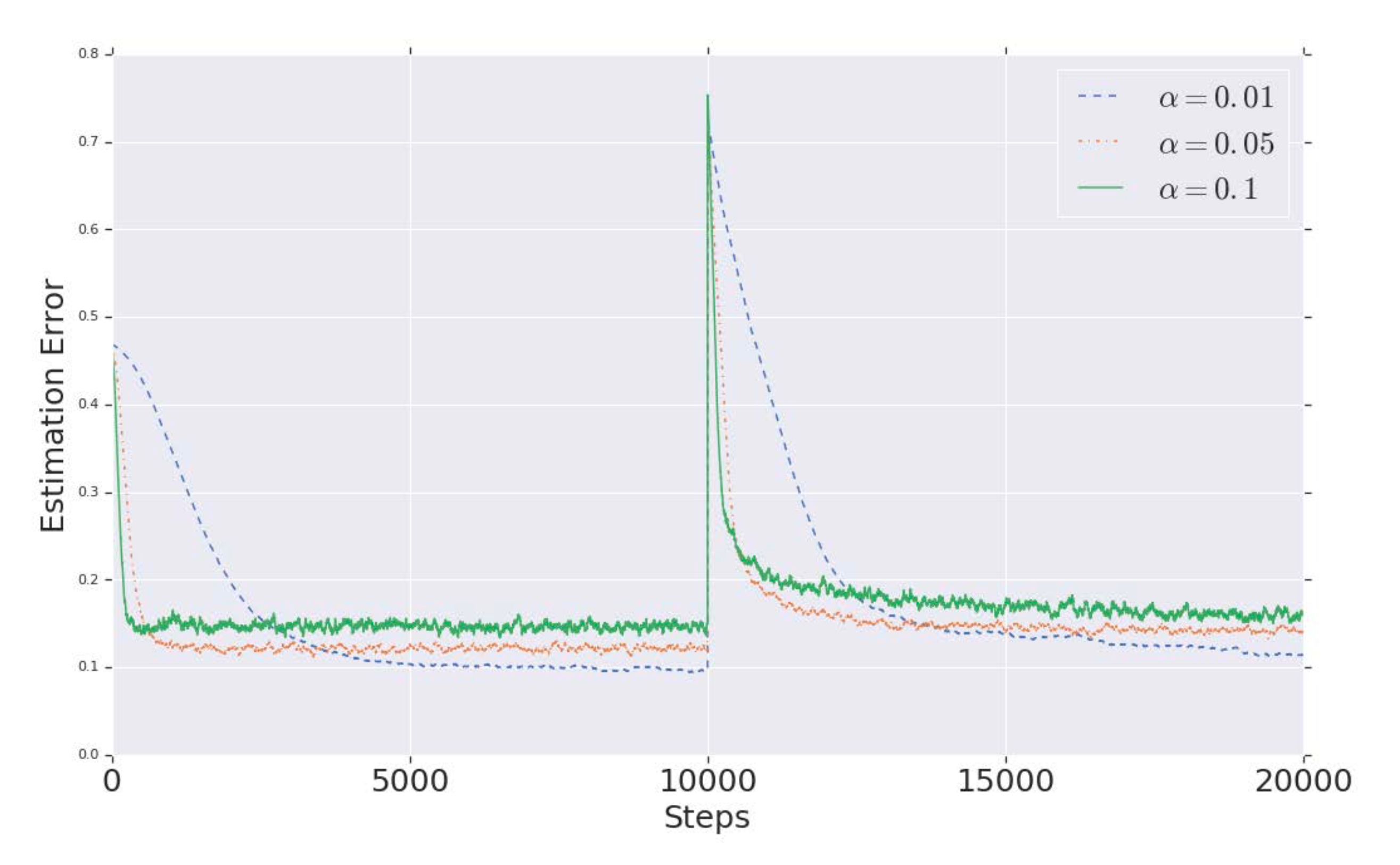
Frequency estimation errors for various learning rates \(\alpha\). And the distribution is switched at step \(t = 10000\).

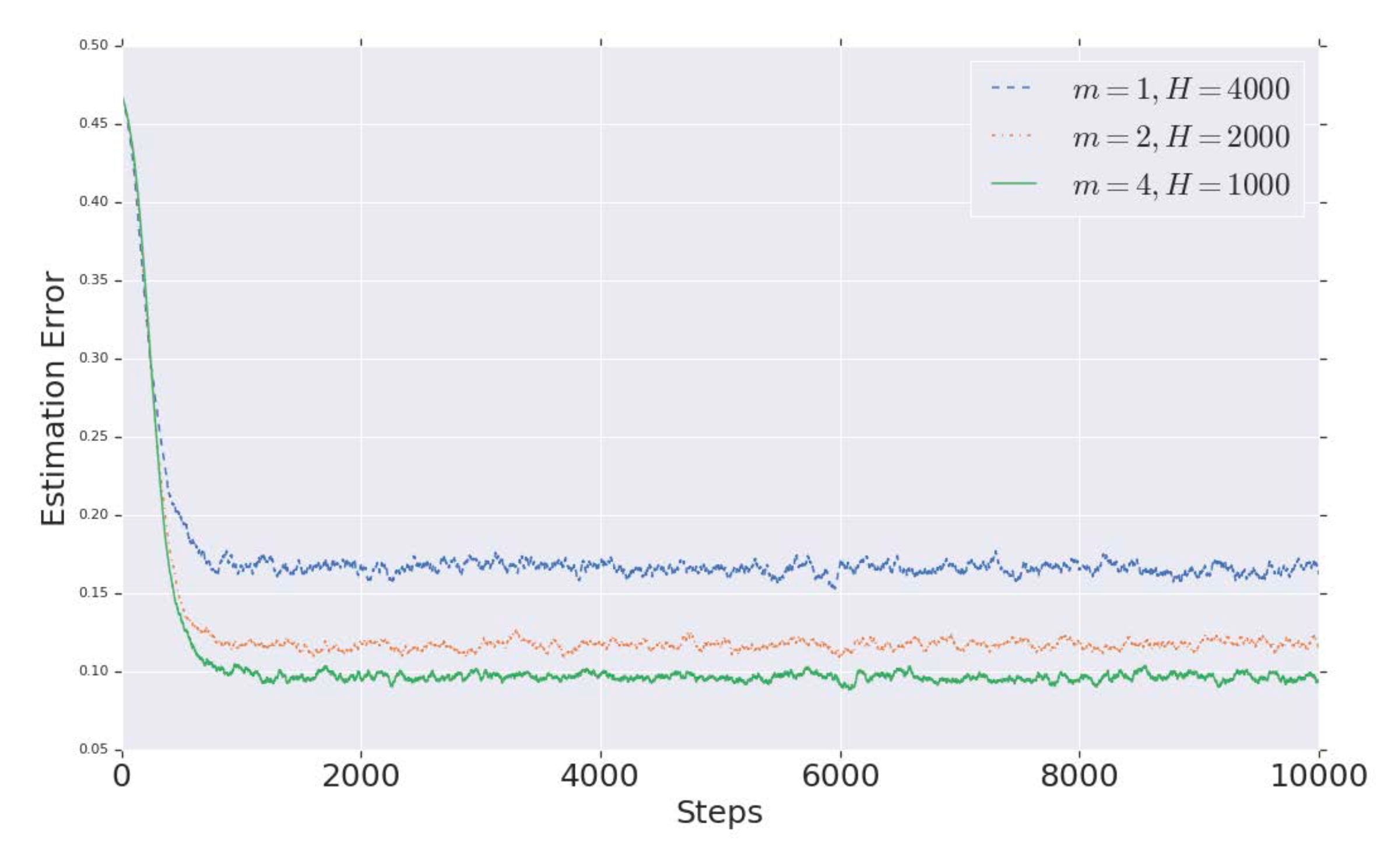
Frequency estimation errors for various number of hash functions \(m\).

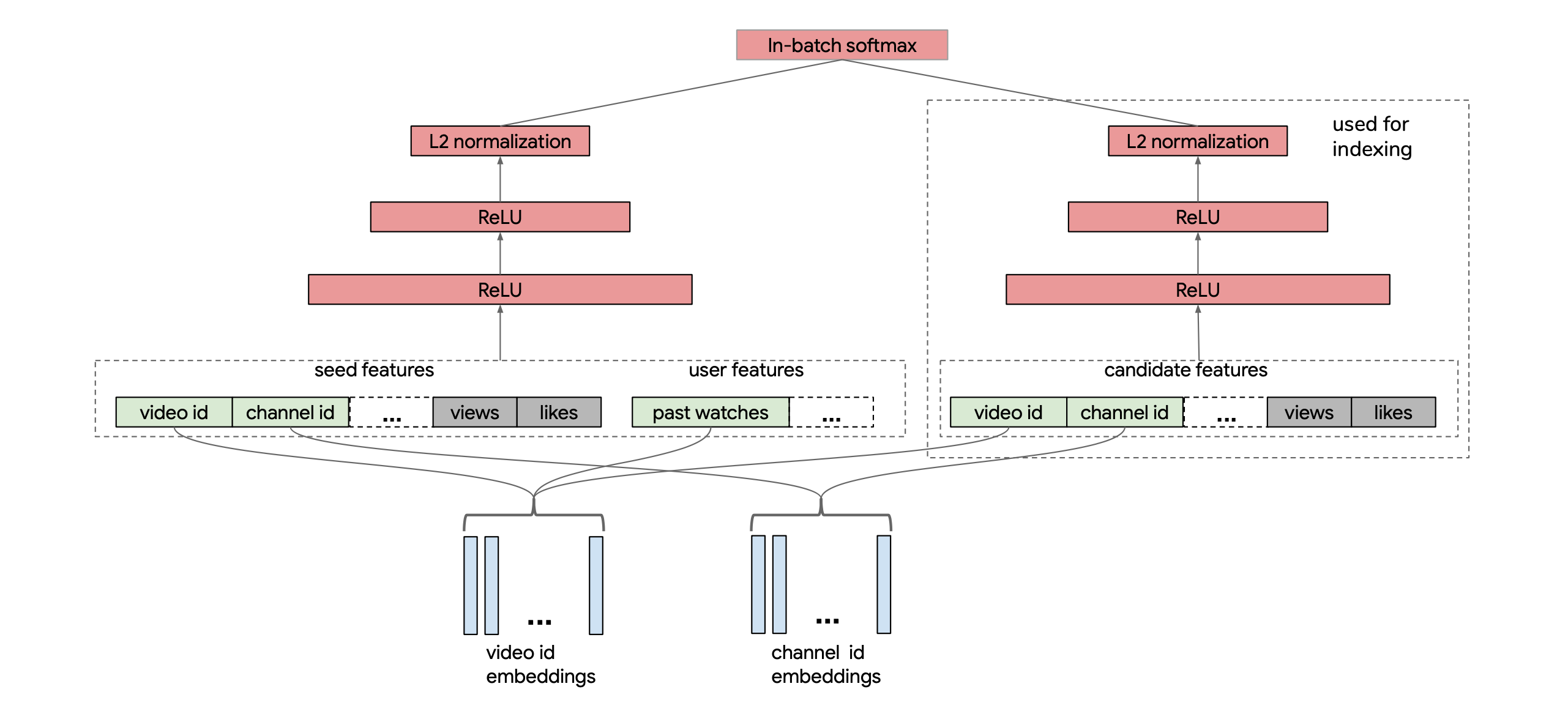
Below is an illustration of the neural retrieval model for YouTube. Plese refer to the paper for more details and experiments.

Reference

• [1] Bengio, Yoshua, and Jean-Sébastien Senécal. “Adaptive importance sampling to accelerate training of a neural probabilistic language model.” IEEE Transactions on Neural Networks 19.4 (2008): 713-722.
• [2] Blanc, Guy, and Steffen Rendle. “Adaptive sampled softmax with kernel based sampling.” International Conference on Machine Learning. 2018.
• [3] Hidasi, Balázs, et al. “Session-based recommendations with recurrent neural networks.” arXiv preprint arXiv:1511.06939 (2015).